The following note is restricted to the most basic problems which Claudius Ptolemy solved in his earliest astronomical treatise, the Mathematical Composition, or Almagest (c. 141 A.D.). Two basic points are clear:
- Ptolemy’s treatment was indeed adequate in terms of the observational data and limitations (pre-telescopic) of his time;
- Ptolemy chose to focus on problems which could be solved mathematically.
To simplify a complex history, it is accurate to point out that, inasmuch as neither the observable data nor the available mathematical techniques were improved for many centuries, it is hardly surprising that Ptolemaic astronomy survived for nearly 1500 years. The Almagest is to classical astronomy what Euclid’s Elements is to geometry. Both were brilliantly structured synthetic compilations employing efforts of others. Ptolemy drew on the mathematical work of Apollonius and the observations of Hipparchus, many of which seem to have derived from the Babylonians.
A distinguishing characteristic of Ptolemy’s viewpoint (and the same may be said of the Greeks generally, in contradistinction to the Babylonians and Egyptians) was the following: The first astronomical problems deserving solution were overall apparent motions. In other words, first priority was assigned to describing mathematically the orbits of the moon, sun, and the five classically known planets (Mercury, Venus, Mars, Jupiter, and Saturn). Only after this set of general problems had been solved satisfactorily would Ptolemy (or his Greek predecessors) attend to more specific problems such as planetary rising times (Babylonian- type problems) or detailed problems relating to time measurement (Egyptian-type problems).
-
Overall Planetary Orbits
There are two types of astronomical problems–mathematically similar but practically distinct–relating to the solution of overall orbits:
- Sun and Moon: The overall orbits of the sun and the moon must be understood, mathematically, to a surprising degree of accuracy in order to construct a calendar of modest accuracy. The complexity of these motions are too often not understood, and hence the seemingly inordinate amount of time spent on solar and lunar motions by ancient astronomers is misunderstood, or worse, belittled. It is easy to appreciate why so much effort was expended on these problems when it is recognized that even today the theoretical problem of earth-moon-sun motions (one aspect of the 3-body problem) is not fully solved.
- Planetary Orbits: Once again, the Greek approach to understanding the apparent wandering motion of the planets (as opposed to the apparent fixity of the stars) dictated some understanding of their overall orbits, and only secondly the analysis of these results for solutions to specific anomalies in each orbit.
Appreciation of this approach is essential to an understanding of Ptolemaic astronomy. One need only recall how the Babylonians approached planetary problems to realize there were indeed other options, that is, for reasons directly related to their mathematical interests, the Greeks (including Ptolemy) chose one of several viable alternatives.
For historical reasons which must be discussed separately, Ptolemy chose the model of epicyclic motion as his basic mathematical tool. In point of fact, considering the mathematical options available to him, he chose wisely indeed. By its nature, epicyclic motion can describe virtually every conceivable closed curve. For example, this simple device can produce such unrelated closed figures as circles, squares, ellipses, etc.:

An unlimited number of open curves, moreover, can be generated by epicyclic motion.
*Even today, the precise position of the moon relative to the earth is not predictable in theory. For example, on a lunar mission, the data fed to the computers on the basis of which initial injection and mid-course correction angles are established come from radar readings bounced continually off the lunar surface. In other words, the data is gathered empirically, rather than computed in advance through theory.
-
Some Elementary Epicyclic Motions

By the use of one epicycle (E) mounted on a deferent (D) which is concentric to the earth, any moving celestial body may be made to appear as if it were moving on a circular but eccentric orbit. This in turn may be used to describe the appearance of changing velocities of the celestial body. Thus the body appears to an observer on earth to be traveling slowest at apogee (A) and most rapidly at perigee (P).
Notice that the same phenomenon is described without using an epicycle by merely assuming an eccentric deferent.
These apparent changes in velocity were the first basic problem to be described for motions of the sun, moon, and planets.
The second basic problem was associated with the planets themselves. Planets appear to approach stationary points, reverse their direction of travel, then become stationary again, and finally proceed in the original direction of motion once again. This striking phenomenon–called ‘retrograde motion’–could be described simply by a second type of epicyclic motion.
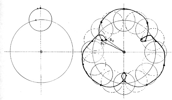
By having the planet travel around the epicycle in the same sense as the epicycle is traveling around the deferent, an observer on earth sees the planet slow down and approach the first stationary point (S1); then go into retrograde motion, next it appears at the second stationary point (S2); and finally it continues in its original sense of motion.
The important mathematical fact here is that by properly assigning (i) the speed of the planet on the epicycle, (ii) the speed of the epicycle on the deferent, (iii) the radius of the epicycle, and (iv) the radius of the deferent, the appearance of retrograde motion could be described for any planet, at any position in the heavens, as often as observation required. In other words, merely by investigating four variables (or, equivalently, two ratios of variables) all apparent retrograde motions were adequately described and were predictable.
Then by combining these two types of epicyclic motion (or eccentric motion for the first type, plus the second type), a planetary theory is constructed which will mathematically describe the two most basic problems in apparent planetary motion: variations in velocity and retrograde motion. Ptolemy’s planetary theory achieved this quite admirably.
At this point in constructing his planetary model, Ptolemy tells us that he is faced with a choice: In order to describe appearances (explicitly, to “save the phenomena,” in Platonic terms) he may use either the first type of epicycle model noted above, or its mathematical equivalent, a simple eccentric deferent; either device accounts for apparent changes in planetary velocities. In either case, however, an epicyclic model of the second type must be added in order to account for retrograde motion. Thus, the option is as follows:

Note carefully the relative senses of rotation. At present the most important facts are (l) that Ptolemy recognized the mathematical equivalence of these two models, and (2) that Ptolemy consciously chose (I) for its ‘mathematical simplicity’ with apparent lack of concern for the actual situation in the physical heavens. Certainly the recognition that he was free to use either (I) or (II) indicates that arguments concerning ‘physical reality’ were not considered at this juncture. In sum, Ptolemy chose to define the problem of describing apparent planetary motions as a mathematical problem, that is, as the problem of constructing a mathematical model by means of which planetary positions (past, present, and future) might be computed and predicted. He aimed at geometrical description with little concern for physical explanation.
One further complication arose. Without explaining to his readers how the discovery was made, Ptolemy nevertheless proceeds to tell us that model (I) is not quite sufficient. In order for (I) to lead to satisfactory computational results, we may not–unfortunately*–conceive of the center of the epicycle as traveling around the center of the deferent at a uniform rate; this leads to erroneous results. Yet the underlying Platonic Dictum of ‘explanations’ in terms of uniform, circular motions (or compounded circular motions) around a central point was apparently so ingrained in Ptolemy’s thought processes that his reaction to the dilemma was to find some other point from which the motion of the center of the epicycle could be considered uniform. This point is the famous punctum aequans, or equant point.
In the final model (m) then, the planet (P) is conceived as traveling uniformly around its epicycle, while the center of the epicycle (on its deferent) travels uniformly around the equant (E), which is situated on the apogee-perigee line of the deferent at the same distance (e) away from its center as is the earth, but in the opposite direction:
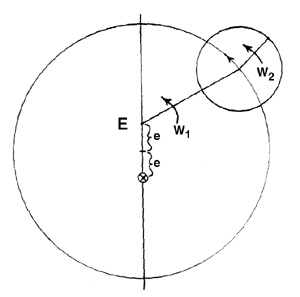
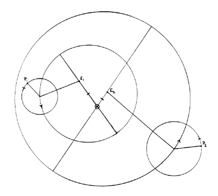
w1 and w2 are constant angular velocities, but here of course w1 is not equal to w2 Note: (1) This general scheme was found by Ptolemy to work for all of the planets except Mercury (cf. (2) infra). However–and this is extremely important in understanding the overall model–the equant points (En) are different points in space for each planet. This point is illustrated in the following diagram, employing only two planets (Pn):
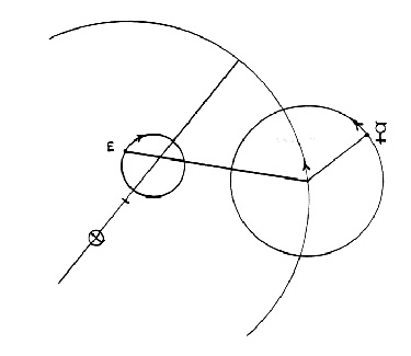
(2) In the case of Mercury, Ptolemy found he could not allow even the equant to be stationary: The equant had to revolve on a completely separate auxiliary circle:
*This would later turn out to be the principal objection of Copernicus to the Ptolemaic planetary scheme.
These notes illustrate only the rudiments of Ptolemaic planetary models. In particular, we have shown only in broad outline how planetary motions in longitude could be described. In addition, the orbits of each of the planets is at a small but easily measurable angle to the plane of the ecliptic. Additional geometrical devices must be introduced to account for observed motions in latitude. Hence, the various deferents and epicycles are at different angles to the ecliptic, requiring still additional tables for computing at any given time the latitude of any planet.
-
Lunar Theory
Ptolemaic lunar theory is an excellent example of the Greek mathematical mind at work. Ptolemy had, first of all, inherited a rather crude epicyclic lunar model from Hipparchus. Hipparchus had known at least of the first, or simple, variation in the moon’s velocity. Perhaps he knew more. In any event, he apparently succeeded in accounting for only this first variation. He did this by using an epicyclic motion of the first type (cf. above).
Ptolemy realized that this model merely approximated actual lunar longitudinal motion. In particular, Hipparchus’ model worked fairly well when the moon was near, or at, conjunction or opposition, with the mean sun. But at quadratures, its accuracy was poor. Ptolemy’s subsequent investigation led to his discovery of the second variation (or inequality), called “evection” by modern astronomers. Briefly, this required that the moon’s epicycle be pulled closer to the earth (in order to appear to be traveling faster than would otherwise have been the case) as the moon’s epicycle approached quadrature with the mean sun. All of this, naturally, made Ptolemy’s lunar tables rather complex. Yet the accuracy gained over earlier tables must have been enormous. They remained in general use until well after the time of Copernicus. It may be remarked, parenthetically, that Copernicus’ lunar tables were–in theory–slightly more accurate than Ptolemy’s; but this accuracy was gained only at the expense of using two epicycles rather than one.
The following three diagrams suggest the sophistication of Ptolemy’s lunar model.
Lunar Diagrams
- Hipparchus’ Model: Single epicycle, producing an eccentric, circular orbit.

- Ptolemy’s Model: When in quadrature to the Mean Sun, the epicycle is ‘pulled in’ toward the earth a maximum distance. This is accomplished by another auxiliary circle and what we can visualize as a rigid ‘connecting rod’ (indicated by the double line). This can be visualized best by several diagrams showing the epicycle at different positions. (Ptolemy’s relative dimensions, of course, cannot be illustrated accurately in these small diagrams).
II.1 and II.2

II.3

Note: Since, as noted above, actual relative lunar dimensions cannot be maintained in such small drawings, the Moon appears in II 3 not to be at quadrature. Actually, it would be very close to line X Y if the dimensions were as Ptolemy’s tables require.
II.4
In IL 3 the epicycle’s center is the closest it ever gets to the Earth. Now, 90° later, it is pushed back out to the original deferent. 90° from this position it is again pulled in to its closest position to the Earth. - The computed Ptolemaic lunar model, showing the fluctuating apogee of the epicycle:
The final lunar model, as presented in the Almagest, is represented in diagram III. The overall orbit of the center of the moon’s epicycle is roughly the inner ovoid curve. If the proper Ptolemaic radial dimensions could be shown, it would be seen that this orbit is very nearly an ellipse. Similarly, the overall orbit of the moon in this model is close to an ellipse. It is for this reason the model worked so well for calendaric purposes, eclipses, and so forth. Ptolemy, however, did not seem to realize that he was using an essentially elliptical orbit. The improvement made by Copernicus with double epicycles (one of which merely replaces Ptolemy’s auxiliary circle and ‘connecting rod’) was an even closer approximation to an ellipse.
The angle ‘a’, called ‘anomaly,’ measures the angular distance of the moon from the apogee of its epicycle. Ptolemy found that this angle–which one must be able to look up in a table in order to find the ‘true’ moon after finding the ‘mean’ moon (= center of epicycle)–must be measured from a ‘fluctuating apogee’ (A), rather than from Hipparchus’ apogee (= extension from through the center of the epicycle), or the point A’ which is the extension of the connecting rod.
The line from the epicycle’s center to A clearly fluctuates–hence the term ‘fluctuating apogee’ –since it is constructed through the center of the epicycle from an imaginary point 180° away from the end of the connecting rod on the auxiliary circle. Since this device is not otherwise motivated theoretically in the text, one can only conclude that Ptolemy discovered its necessity empirically.
One must further remember that, just as in the case of planetary orbits, the moon’s latitudinal motion had also to be computed. That part of the model is omitted here.
- Hipparchus’ Model: Single epicycle, producing an eccentric, circular orbit.
-
Ptolemy’s Star Catalogue (ALMAGEST)
1028 stars are listed by longitude and latitude. Three of these are duplicates. Despite the often repeated assertion that Ptolemy’s Star Catalogue (end of Book VII and beginning of Book VIII of the Almagest) was merely that of Hipparchus (brought up-to-date by correcting for precession of the equinoxes at the rate of 1° per century), Vogt (1925) has shown that this is not likely, that is, that Ptolemy’s Catalogue seems to have been separate and original.
This summary is adapted from an unpublished ditto handout by the late W.D. Stahlman. The text has been revised, illustrations have been redrawn and corrected by R.A. Hatch.